Practical Data Science

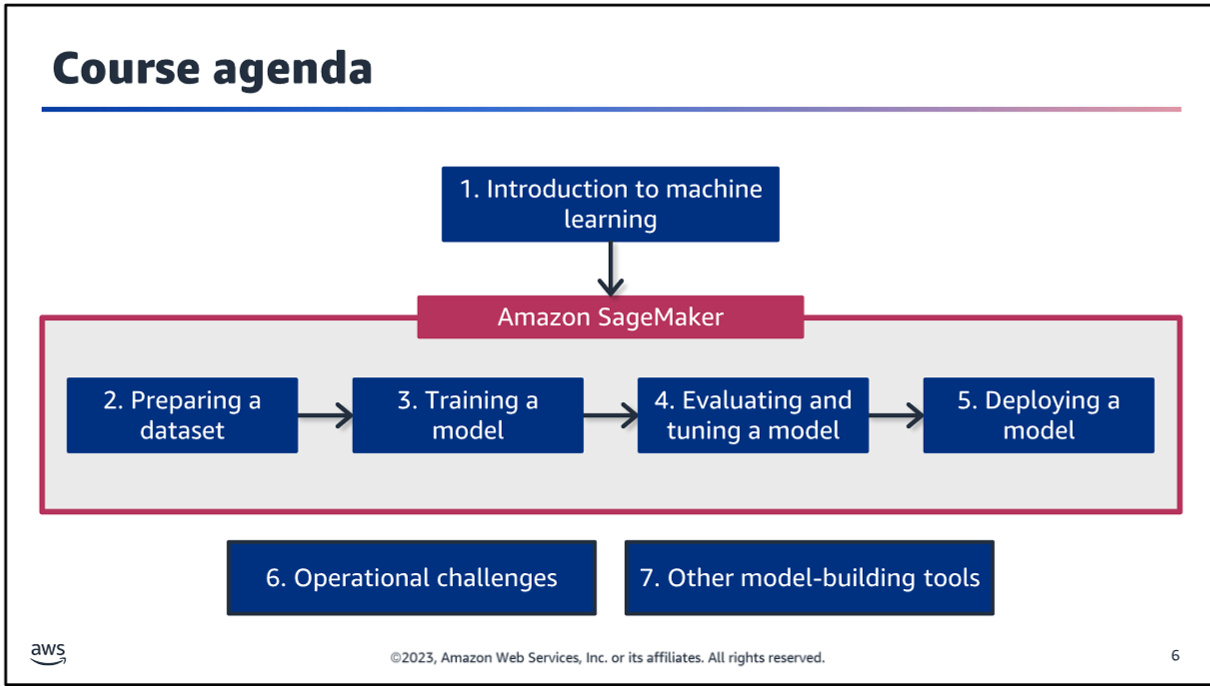
Common ML use cases

• Classification: Predicting a category
• Regression: Predicting a number
• Clustering: Finding groups in data
• Anomaly detection: Finding outliers

ML model benefits

• identify patterns: ML models can identify patterns in data that humans can't

• Minimize human error: ML models can make predictions without human intervention

• Can become more accurate over time: ML models can learn from new data and improve their predictions

• variety of data: ML models can handle a variety of data types, including images, text, and numbers

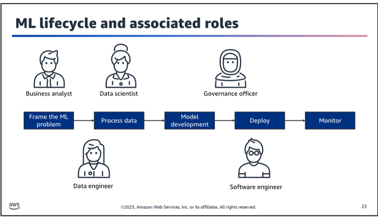
How to build a Quality dataset Journey

Once you have a dataset, you can start building a machine learning model. The process of building a machine learning model can be broken down into the following steps:

1. Frame the problem: What are you trying to predict? What data do you have available to make predictions?

2. Prepare the data: Clean the data, and split it into training and test sets.

3. Model Development: Train a machine learning model on the training data.

4. Deploy the model: Use the model to make predictions on new data.

5. Monitor the model: Keep track of how well the model is performing, and update it as needed.

Correlation Matrix

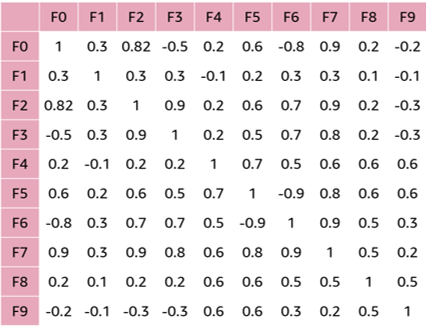
A correlation matrix is a good tool to quantify the linear relationship among the variables as it conveys both the strong and weak linear relationships among numerical variables. It is a k by k matrix, where k is the number of columns in your data including the target. Each cell is populated with the corresponding correlation between the corresponding column variables.

The matrix shown is for a dataset with 9 features, F0 - F9. The matrix displays the correlation between each pair of features. The closer a value is to 1 or -1, the more linear is the relationship. A value close to or equal to 0 shows no linear relationship.

The analyzed dataset may then be filtered and adjusted to improve the quality for training and evaluating a model. Such actions may be dropping some features when they are highly correlated to others or filtering the dataset so that features and target are more balanced.56

Data considerations for model training

• Data size and quality: The more data you have, the better your model will be. However, more data also means more time and resources to process it. You should also consider the quality of your data. If your data is noisy or has missing values, your model will be less accurate.

• Representativeness: Your data should be representative of the problem you are trying to solve. For example, if you are trying to predict the price of a house, your data should include information about the size, location, and condition of the house.

Dission Tree

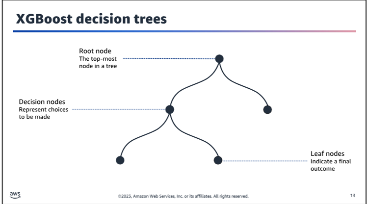
XGBoost

• XGBoost is a popular machine learning library that is used for building decision trees. It is known for its speed and accuracy, and is often used in machine learning competitions.

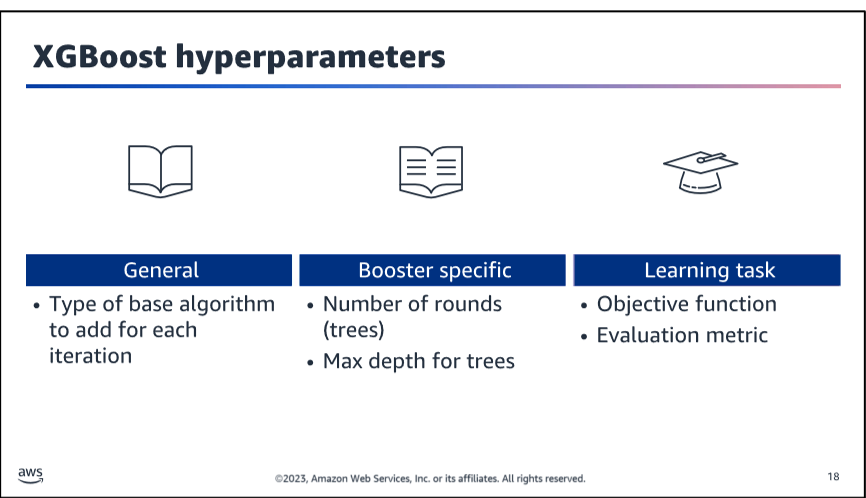
XGBoost Hyperparameters

• alpha: L1 regularization term on weights. Increasing this value will make model more conservative.

• eta: Step size shrinkage used in update to prevents overfitting. After each boosting step, we can directly get the weights of new features, and eta shrinks the feature weights to make the boosting process more conservative.#### XGBoost Hyperparameters

• min_child_weight: Minimum sum of instance weight (hessian) needed in a child. If the tree partition step results in a leaf node with the sum of instance weight less than min_child_weight, then the building process will give up further partitioning. In linear regression task, this simply corresponds to minimum number of instances needed to be in each node. The larger, the more conservative the algorithm will be.

• num_round: The number of rounds for boosting. This is the number of boosting iterations. The larger, the more accurate the model will be, but also the longer it will take to train.

• max_depth: Maximum depth of a tree. Increasing this value will make the model more complex and more likely to overfit.

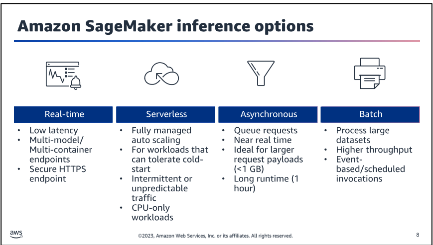
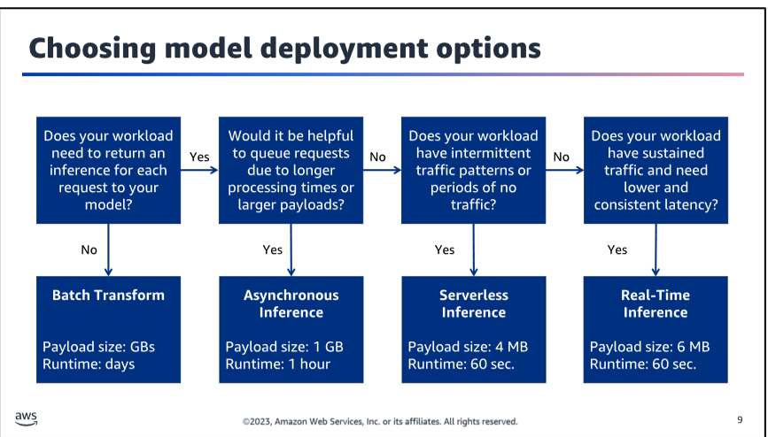
Amazon Sage Maker inference options

• Real-time inference: Use a model to make predictions on new data in real time. This is useful when you need to make predictions quickly, such as in a web application.

• Batch inference: Use a model to make predictions on a large batch of data. This is useful when you need to make predictions on a large dataset, such as a log file or a database.

• Asynchronous inference: Use a model to make predictions on new data, and then store the predictions in a database. This is useful when you need to make predictions on new data, but don't need the predictions immediately.

• Batch inference: Use a model to make predictions on a large batch of data. This is useful when you need to make predictions on a large dataset, such as a log file or a database.

Choosing model deployment options

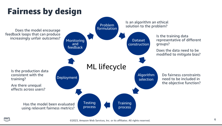
ML lifecycle

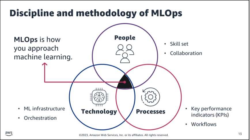
Methodology of MLOps

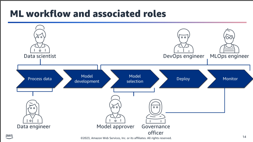
Workflow and associated roles

SageMaker Studio for ML Lifecycle

SageMaker Studio is a web-based IDE for building, training, debugging, deploying, and monitoring ML models. It supports the full ML lifecycle with a unified visual interface.

Features

• Write and run code in Jupyter notebooks
• Build and train ML models
• Deploy models and monitor performance
• Track and debug ML experiments

Architecture

SageMaker Studio notebooks have a two-layered architecture:

1. JupyterApp: Provides the JupyterLab IDE user experience
2. Kernel App: Runs notebook code cells, defines image and compute instance type

This architecture uses a gateway application pattern to connect JupyterApp and Kernel App.

Key Benefits

• Fast: Launch instances in under 2 minutes
• Convenient: Amazon SageMaker Python SDK pre-installed, multiple kernels available
• Comprehensive: Build, train, debug, track, monitor, and view experiments
• Sharable: Read-only copy includes dependencies
• Scalable: Fully elastic compute resources
• Persistent: View and share notebooks even when instances or kernels are stopped
• Scheduled: Run notebooks on demand or on a fixed/custom schedule
• Flexible: Select different kernel images and instance types

SageMaker Data Wrangler

SageMaker Data Wrangler is a tool that helps to complete each of the key ML data preparation workflow tasks. It includes data loading, cleaning, exploring, and visualization with little to no code.

Key capabilities of SageMaker Data Wrangler include the following:

• Select data from multiple data sources and semi-structured data formats.
• Automatically verify data quality and detect abnormalities.
• Understand data with visualization templates.
• Transform data with 300+ built-in transformations plus the ability to author custom transformations.
• Quickly estimate ML model accuracy and diagnose issues before models are deployed into production.
• Automate ML data preparation workflows.# SageMaker Data Wrangler

SageMaker Data Wrangler is a tool that helps to complete each of the key ML data preparation workflow tasks. It includes data loading, cleaning, exploring, and visualization with little to no code.

Key capabilities of SageMaker Data Wrangler include the following:

• Select data from multiple data sources and semi-structured data formats.
• Automatically verify data quality and detect abnormalities.
• Understand data with visualization templates.
• Transform data with 300+ built-in transformations plus the ability to author custom transformations.
• Quickly estimate ML model accuracy and diagnose issues before models are deployed into production.
• Automate ML data preparation workflows.# SageMaker Data Wrangler

SageMaker Data Wrangler is a tool that helps to complete each of the key ML data preparation workflow tasks. It includes data loading, cleaning, exploring, and visualization with little to no code.

Key capabilities of SageMaker Data Wrangler include the following:

• Select data from multiple data sources and semi-structured data formats.
• Automatically verify data quality and detect abnormalities.
• Understand data with visualization templates.
• Transform data with 300+ built-in transformations plus the ability to author custom transformations.
• Quickly estimate ML model accuracy and diagnose issues before models are deployed into production.
• Automate ML data preparation workflows.

Regression Problem metrics

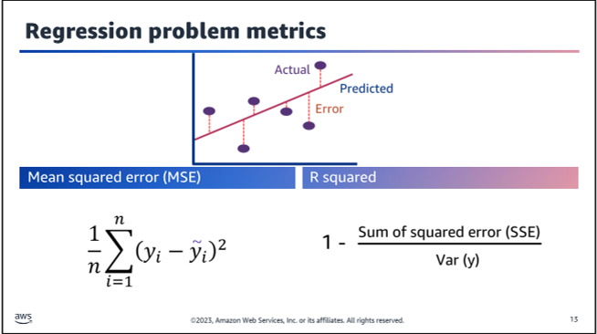
1. Mean Squared Error (MSE):

   • MSE measures the average squared difference between the predicted values and the actual values.
   • It provides an understanding of the magnitude of the errors made by the model.
   • Lower MSE values indicate better model performance.
   • MSE is sensitive to outliers, as squaring the errors magnifies the effect of large errors.

2. R-squared (R²):

   • R² measures the proportion of the variance in the target variable that is explained by the independent variables in the model.
   • It ranges from 0 to 1, with a value closer to 1 indicating a better fit of the model to the data.
   • R² provides an intuitive interpretation of the model's goodness-of-fit.
   • However, R² tends to increase as more variables are added to the model, even if those variables are not significant, leading to potential overfitting.

3. Adjusted R-squared (Adj. R²):

   • Adjusted R² is a modified version of R² that accounts for the number of independent variables in the model.
   • It aims to penalize the addition of insignificant variables, reducing the risk of overfitting.
   • Adjusted R² only increases if the new variable improves the model's performance more than would be expected by chance.

When evaluating a regression model, it is recommended to consider both MSE and R² (or Adjusted R²) to get a comprehensive understanding of the model's performance and potential overfitting issues.

Python Code:

from sklearn.metrics import mean_squared_error, r2_score
from sklearn.linear_model import LinearRegression
import numpy as np

# Example data
X = np.array([[1], [2], [3], [4], [5]])
y = np.array([2, 4, 5, 4, 5])

# Create and fit a linear regression model
model = LinearRegression()
model.fit(X, y)

# Make predictions
y_pred = model.predict(X)

# Calculate mean squared error
mse = mean_squared_error(y, y_pred)
print("Mean Squared Error:", mse)

# Calculate R-squared
r2 = r2_score(y, y_pred)
print("R-squared:", r2)

# Calculate Adjusted R-squared (assuming single feature)
n = X.shape[0]  # Number of observations
p = 1  # Number of features (assuming single feature)
adj_r2 = 1 - (1 - r2) * ((n - 1) / (n - p - 1))
print("Adjusted R-squared:", adj_r2)

In this example, we generate some example data, create and fit a linear regression model, and then calculate the mean squared error, R-squared, and Adjusted R-squared using functions from the sklearn.metrics module.

Note that the Adjusted R-squared calculation assumes a single feature (independent variable). If you have multiple features, you would need to adjust the formula accordingly.

More about sage Maker Built in Algorthim

Amazon Sage MakerAmazon Sage MakerSage Maker Built-in Algorithms Linear Learner Linear Learner is a supervised learning algorithm that can be used for both classification and regression tasks. It's a simple yet powerful algorithm that works well for high-dimensional, sparse data. Key Features**: - Linear Models: It supports both linear regression and binary/multiclass classification. - Automatic Tuning: It automatically tunes the model complexity based on the input data. - Scalability: It can handle large datasets and